
Summary
Two highly correlated distributions ($S1$, $S2$) are created
from scratch. A scatter plot of both distributions distributions is created,
with values on the x-axis from $S1$ and values on the y-axis from $S2$, to
display what collinearity looks like. Covariance along with the prerequisites
that need to be met for it to be a suitable metric, is first explored as a
metric to spot collinearity. The mathematical formula and a shortcut for
calculating it are presented. The second metric is the Pearson Correlation
Coefficient. It is described much like the Covariance, along with an
description the possible values of the correlation coefficient $r$. The articles
concludes with an example of how the Pearson Correlation Coefficient can be
used in a hypothesis test to determine, if $S1$ and $S2$ are at all correlated
with each other.
Multicollinearity
Covariance and the Pearson Correlation Coefficient: How to Spot
Multicollinearity between random variables.
Multicollinearity is a statistical concept, that describes the phenomenon of
several independent variables, that are part of a multiple regression model, are
linearly correlated with each other. In this article we mention two metrics,
that can be used to test for collinearity between two random variables. The
metrics work on a per-pair or independent variables basis and so can be
illustrated by using two random variables S1 and S2 in the following.
There are several reasons, why having Multicollinearity among several independent variables can cause problems. Some of them are:
- The presence of Multicollinearity undermines the statistical significance of an independent variable.
Multiple linear regression models are often used for their easy to explain relationship between the independent variables and the dependent variable. One important metric when describing this relationship is, whether the impact of an independent variable on the dependent variable is statistically significant. If this is the case, then the coefficients, that a model assigns to each independent variable $X_{i}$ is proportional (in case of a continuous variable $X_{i}$ and dependent variable $Y_{i}$) to the impact that the variable has on the dependent variable. Boolean variables can be used to describe other relationships between independent and dependent variable.. That is, if the model does not suffer from Multicollinearity among other problems, that can undermine this relationship.
Creating Suitable Samples
Importing the needed modules and functions and setting a seed, so results are comparable across different executions of the code.
1
2
3
4
5
6
7
8
9
10
11
12
13
14
15
16
17
18
19
import matplotlib.pyplot as plt
# Generate related variables
from numpy import mean, std, cov
from numpy.random import randn, seed

plt.style.use('science')
seed(42)


S1 = 20 * randn(1000) + 100
S2 = S1 + (10 * randn(1000) + 50)
print(f'mean, std of S1: {mean(S1)}, {std(S1)}')
print(f'mean, std of S2: {mean(S2)}, {std(S2)}')
plt.scatter(S1, S2, s=2)
plt.xlabel('Distribution of S1')
plt.ylabel('Distribution of S2')
plt.title('Correlation between S1 and S2')
plt.show()
1
2
mean, std of S1: 100.38664111644651, 19.574524154947085
mean, std of S2: 151.09500348893803, 21.605231186428536
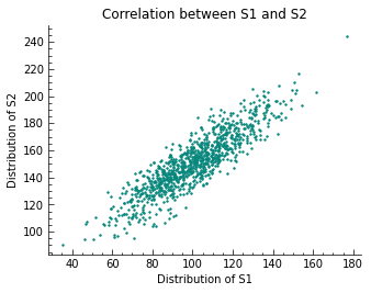
As designed, the two samples S1 and S2 are positively correlated with one another, as visualized in the scatter plot. It must be said, that all the methods mentioned in this article only explain the linear part of the statistical relationship between random variables.
Covariance
To quantify the relationship between to variables, that have a linear relationship, the empirical covariance is often used. It is calculated as the average of the product between the values from each sample, where the values have been centered (had their means subtracted). The calculation of the sample covariance is done using the following formula:
\[cov_{XY} := \frac{1}{n} \sum_{i=1}^{n} (\,x_{i} - \bar{x})\, (\,y_{i} - \bar{y})\, \iff\,\, \overline{xy} - \bar{x} \bar{y}\]$n$ is the number of values. Given the scatter plot of all $\left(x_{i},y_{i}\right)$ tuples with $x_{i}\in\mathrm{S1}$ and $y_{i}\in\mathrm{S2}$, a positive value for $cov(\,x,y)\,$ is expected. The relationship between the two distributions is of linear nature and so the covariance should be a good measure for how they are correlated.
1
2
3
cv = cov(S1, S2)
cv
1
2
array([[383.54554143, 375.65364293],
       [375.65364293, 467.25326789]])
The covariance matrix values of ~375.65 show, that there is a strong positive correlation between S1 and S2. A strong sign for Multicollinearity between the two distributions. This would have to be addressed before training a linear regression model, among others for example. Given the design, there was no problem with satisfying the prerequisites that need to be met, in order for the covariance to be a good measurement for the relationship between two or more distributions found in a dataset (on a per-pair testing basis). Generally, explanatory variables are tested in this regard.
Pearson Correlation Coefficient
Another frequently used measure to determine whether 2 random variables are correlated or not and if, how strongly, is the empirical correlation coefficient, also known as the Pearson correlation coefficient. It utilizes the covariance value and divides it by the product of the standard deviations of the random variables. It is given by:
\[r_{XY} := \frac{cov_{XY}}{s_{X}s_{Y}}\]The domain of $r$ is $[-1,1]$, with:
| value $r$ | counterpart | bivariate relationship |
|---|---|---|
| 0 | - | none |
| 0.1 | -0.1 | weak |
| 0.3 | -0.3 | moderate |
| 0.5 | -0.5 | strong |
| 1 | -1 | perfect |
The plot of the values of two random variables ranges from close to a line with a negative slope, to close to a line with a positive slope. Values of $r\le-0.5$ and $r\ge0.5$ tend to signal a strong correlation in the respective direction. One of the good characteristics, that $r$ has, is that its value does not change, if the random variables are subjected to a linear transformation. That means, that the scale of the random variables or the difference in scale do not affect its value. The sign of $r$ is the same as for $cov$, a difference is that it is normed to the domain of $[-1,1]$
unlike the $cov$ which returned a value of ~375.65 for our example.
Hypothesis Testing
In the next section, the pearsonr function from scipy is used to compute $r$
for the example. We conclude with a hypothesis test, asking whether random
variables S1 and S2 are positively correlated.
1
2
3
4
5
6
7
8
9
10
11
12
13
14
from numpy.random import seed
from scipy.stats import pearsonr

seed(42)
# calculate values
corr, p = pearsonr(S1, S2)
print(f'The Pearson correlation coefficient for S1 and S2 is {corr}\n')
# significance given p value and 0.05 threshold α
alpha = 0.05
if p > 0.05:
	print(f'p-value of {p} is greater alpha={alpha}, H0 is kept.')
else:
	print(f'p-value of {p} is smaller alpha={alpha} and H0 is rejected.\nThere is correlation between the two, given threshold alpha={alpha} on a one-tailed test.')
1
2
3
4
The Pearson correlation coefficient for S1 and S2 is 0.8873663623612615

p-value of 0.0 is smaller alpha=0.05 and H0 is rejected.
There is correlation between the two, given threshold alpha=0.05 on a one-tailed test.
The results show, that the positive linear relationship between the random variables S1 and S2 was confirmed by $r$. The two metrics $r$ and $cov$ gave correct predictions in regard to the correlation.
This marks the end of this educational article.