Questionnaire Chapter 04

How is a grayscale image represented on a computer? How about a color image?
How are the files and folders in the MNIST_SAMPLE dataset structured? Why?
Explain how the “pixel similarity” approach to classifying digits works.
What is a list comprehension? Create one now that selects odd numbers from a list and doubles them.
What is a “rank-3 tensor”?
What is the difference between tensor rank and shape? How do you get the rank from the shape?
What are RMSE and L1 norm?
How can you apply a calculation on thousands of numbers at once, many thousands of times faster than a Python loop?
Create a 3×3 tensor or array containing the numbers from 1 to 9. Double it. Select the bottom-right four numbers.
What is broadcasting?
Are metrics generally calculated using the training set, or the validation set? Why?
What is SGD?
Why does SGD use mini-batches?
What are the seven steps in SGD for machine learning?
How do we initialize the weights in a model?
What is “loss”?
Why can’t we always use a high learning rate?
What is a “gradient”?
Do you need to know how to calculate gradients yourself?
Why can’t we use accuracy as a loss function?
Draw the sigmoid function. What is special about its shape?
What is the difference between a loss function and a metric?
What is the function to calculate new weights using a learning rate?
What does the DataLoader class do?
Write pseudocode showing the basic steps taken in each epoch for SGD.
Create a function that, if passed two arguments [1,2,3,4] and 'abcd', returns [(1, 'a'), (2, 'b'), (3, 'c'), (4, 'd')]. What is special about that output data structure?
What does view do in PyTorch?
What are the “bias” parameters in a neural network? Why do we need them?
What does the @ operator do in Python?
What does the backward method do?
Why do we have to zero the gradients?
What information do we have to pass to Learner?
Show Python or pseudocode for the basic steps of a training loop.
What is “ReLU”? Draw a plot of it for values from -2 to +2.
What is an “activation function”?
What’s the difference between F.relu and nn.ReLU?
The universal approximation theorem shows that any function can be approximated as closely as needed using just one nonlinearity. So why do we normally use more?

$g_{j}$ is a nonlinear activation function associated with unit $j$ and ${in}_{j}$

import string
import numpy as np
import torch
from fastai.vision.all import *

1.

How is a grayscale image represented on a computer?
How about a color image?

Both are represented by a number of pixels, pixels are the most basic foundation, that every digital has. Pixels form rows and columns - an image is like a matrix in most cases, as its shape is rectangular. It can have ‘any’ 2 dimensional shape in theory, however.
Pixels are used to calculate the dimensions, the most elemental measure, assuming all pixels have the same size - not the case in reality. Size of pixels can vary greatly and differs across camera sensors for example. Both, grayscale and color images have a brightness value for each pixel in the image. An important difference between a grayscale and an actual ‘black and white’ (bw) image is that every pixel in a bw image can only have one of two values. Assuming, the grayscale image has brightness values from completely black to completely white, given by the integer range of 0-255, then each pixel in the bw image either has a value of 0 or 255. A threshold is set by which it is determined, if a pixel is converted to 0 or 255. The bw image therefore only needs a 1-bit representation (monochrome) and as such has a very small file size in general, compared to any other bit-depth. The grayscale image on the other hand has pixels that are in the range between and including the borders of 0-255. The grayscale image, depending on how much information about each pixel’s luminosity value is saved, can use 8-bit grayscale color depth or even 16-bit. The file size compared to the same image in monochrome increases, as a higher color depth is chosen. The darkest value possible is black and is usually found on the left edge of the histogram, while the brightest value is completely white found on the right edge of the histogram. These mark the maxima when it comes to the borders of the brightness values. There are two very important properties, associated with either of the two extremes, referred to as ‘clipping’. Clipping occurs, when the luminosity value of a pixel is either 0 or 255. If the clipping was not introduced by post-processing and there is no other version of the image available, that holds another value than 0 or 255 for that pixel, there is no way to recover the damage done by clipping. In this regard, color images and grayscale images are the same. The color image has no color values stored in any of the RGB channels, assuming any RGB, color space. However, in the case of a color image, there is a chance, that not all of its three color channels show a value of 255, that is Red/Green/Blue = 255/255/255. This is why the RGB histogram should be configured to show the distribution for the three channels. There are impressive reconstructions, that can be made using the individual channels. It is the same for pixels with value 0. A color image usually has a vector of the primary colors (RGB) for each pixel. The vector consists of a value for the red, green and blue channel. Together these three elements of the vector can represent a large color space, depending on the color depth and camera sensor among other factors. Color space, e.g., sRGB, Adobe RGB. There are different metrics used to represent the color of an image. The above was RGB == Red Green Blue channels. There are many others like CMYK for example.

2.

How are the files and folders in the MNIST_SAMPLE dataset structured?
Why?

The structure is the following:
- valid
- labels.csv
- train
The structure makes it easy for one to define the validation set and test set, tell the model which labels there are and how they are assigned to the data.

3.

Explain how the “pixel similarity” approach to classifying digits works.

The approach, outlined here is only defined for the case of 2 classes, where the model has to predict whether an image belongs to class 1 (image shows a digit 3) or to class 2 (image shows a digit 7). All images have a square size of 28x28 px.
For both classes, a mean pixel value, representing the ‘ideal’ 3 and 7 respectively is calculated by:

Stacking all images from one class found in the train dataset.
Converting each number, that represent the brightness of a pixel to float, so that all values can be divided by 255. Values were smaller 255 before the division, for all pixels and therefore values between 0 and 1 are created for all pixels.
The mean over all the resulting values between 0 and 1 is created == mean3 and mean7 are created. These mean3/7 values now have dimensions 28x28px and each number (one per row, column coordinates) is the mean for the pixel with these coordinates over all the training set images of that class.
Next, a mechanism to measure the distance between a sample of the same class, and the mean3/7 is created.
The function created calculates the mean absolute error to measure the pixel similarity of mean and sample (same class). Only shown for digit 3, but the same for 7.
MAE(s3,m3) for sample 3 (s3) and mean 3 (m3) is given by: MSE(s3,m3):=(s3-m3).abs().mean()
Another measure for the distance is created. The MSE, mean squared error is used. Calculation is performed using the following formula: MSE(s3,m3):=((s3-m3)**2).mean().sqrt()
The actual predictions for the class of the input image in this method is done by calculating MAE or MSE (only one of the two can be used during an epoch as minimum.)
Assuming, MSE is picked, the prediction for a sample image, that has label 3 ( ss_3) is made by the model by calculating for m3 and m7 respectively:
MSE(ss_3,m3)=((ss_3-m3)**2).mean().sqrt()
The model then compares MSE(ss_3,m3)= 3diff and MSE(ss_3,m7)= 7diff.
It calculates 3diff - 7diff = ss_3d.
- If ss_3d < 0 => 3diff < 7diff and pred = ss_3 is a 3
- If ss_3d > 0 => 3diff > 7diff and pred = ss_3 is a 7
- If ss_3d = 0 => a 50/50 random choice could be used to settle these problematic cases. Or the MAE could be calculated and if that loss-function gives a result that is not 0, it could be chosen over the MSE in these cases.

4.

What is a list comprehension? Create one now that selects odd numbers from a list and doubles them.

l = [2 * n for n in range(20) if n % 2 != 0]
l

[2, 6, 10, 14, 18, 22, 26, 30, 34, 38]

5.

What is a “rank-3 tensor”?

A rank-3 tensor is a list of matrices, since a matrix itself is a rank-2 tensor. That is, since it has 2 axes, as is a list of vectors. E.g.,

rng = np.random.default_rng()
ints = list(rng.integers(0, 10, 5))
rank1 = tensor(ints)
rank2 = tensor([ints, ints])[:, :-2].resize(2, 3)
rank3 = tensor([[ints, ints], [ints, ints]], [[ints, ints], [ints, ints]]).resize(
    1, 20, 2
)
# rank3 = tensor([[ints, ints],[ints,ints]])#[:-2,:] #.resize(18,2)
# rank3 = tensor([[
# for i in zip(range(1,4),['rank'+str(j) for j in range(1,4)]):
for i in zip(range(1, 4), [rank1, rank2, rank3]):
    print(f"rank{i[0]}: {i[1]}, dim: {i[1].ndim}\n")

rank1: tensor([5, 7, 8, 7, 4]), dim: 1

rank2: tensor([[5, 7, 8],
        [5, 7, 8]]), dim: 2

rank3: tensor([[[5, 7],
         [8, 7],
         [4, 5],
         [7, 8],
         [7, 4],
         [5, 7],
         [8, 7],
         [4, 5],
         [7, 8],
         [7, 4],
         [5, 7],
         [8, 7],
         [4, 5],
         [7, 8],
         [7, 4],
         [5, 7],
         [8, 7],
         [4, 5],
         [7, 8],
         [7, 4]]]), dim: 3

6.

What is the difference between tensor rank and shape?
How do you get the rank from the shape?

Tensor rank is equal to the number of axes $\iff$ dimensions a tensor has. The rank of a tensor can be calculated using the ndim method, like so: tensor.ndim (no parenthesis). Examples for an axis/dimension of a rank-1, rank-2, rank-3 tensor are:

rank-1: The number of elements in a tensor vector.
rank-2: In a tensor matrix, the rows and columns both are axes/dimensions. The count of axes is 2 for a matrix, hence it is a rank-2 tensor.
rank-3: A list of tensor matrices has 3 axis. The first two are the ones described in a rank-2 matrix. The third is given by the axis, that goes over all the matrices in the list of matrices. E.g., the set of training images, that are appended to form one list of matrices, each representing one image in the training set.

Tensor shape: is given for each axis, that a tensor has. The shape, is a tuple with the number of elements equal to the tensors rank. Each element in the tuple is equal to the number of elements that are in the axis it represents.

Derive rank from shape: As mentioned in tensor shape, the shape is a tuple of length equal to the tensor’s axes. Therefore, the following relationship holds true for deriving the rank from the shape: $\mathrm{tensor.ndim} \iff \mathrm{len}(\,\mathrm{tensor.shape})\,$

7.

What is the RMSE?
What is the L1 Norm?

RMSE

With $\overrightarrow{\boldsymbol{x}}$ as the mean over all records in the dataset of the independent variable (e.g., a feature vector), $\overrightarrow{\boldsymbol{y}}$the mean over all records of the dependent variable in the dataset (e.g., a multi-class label vector) with both having a length of$N$$. Then, the root mean squared error (RMSE) is defined by:

\[\mathrm{RMSE}=\sqrt{\sum_{i}^{N}\frac{(x_{i}-y_{i})^2}{N}}\]

The definition of the RMSE, is identical to the one of the MSE, except for the last step. The step, where we take the square root of the value, that is equal to the MSE.
In Detail:
The MSE is the mean of the sum of all the squared distances between actual ($x_ {i}$) and predicted ($y_{i}$) values. The distances are also known as residuals, so it is the mean of the squared sum of residuals.

The RMSE then is the square root of the MSE. The square root of the mean of the sums of the residuals.
The characteristics of the two metrics show some differences, that show more or less depending on the data given. The MSE punishes large single residuals much harsher than the RMSE does. Taking the square of the absolute distance between target and predicted label has the effect of treating all residuals equal. The sign of target and predicted value does not matter.

The nominator in the equation is squared, which makes the nominator a polynomial function of second degree. On the other hand, the denominator is a first degree polynomial term. It is obvious, according to l Hospital’s theorem, that the linear term in the numerator, in general, has vanishingly small influence on the function values compared to the quadratic term in the numerator. This relationship is also reinforced by the fact that the values in the numerator are not upper bounded. The denominator, on the other hand, is a constant quantity determined by the size of the data set.

In summary, the MSE penalizes single large deviations between prediction and actual target label very harshly. Consistency, low average deviations do not have a high value if large deviations occur.
This is a summary, in individual cases these characteristics may be absent.

The RMSE weakens the weighting of the quadratic denominator by taking the root of the whole term at the end. It is a metric that represents a trade-off between penalizing large deviations and lack of consistency, in the direction of prioritizing consistency.

L1 norm

The L1 norm is the L1_Loss function here. The function is: $\mathrm{L1_{Loss}}(\,ss_{3},label_{target})\, := |ss_{3} - label_{target}|$ for $ss_{s3}$ one sample of the independent variable, $label_{target}$ the ground truth. It calculates the absolute value of the distance between predicted label and actual target label. The function will only output values, that are not 0 for instances where the predicted label is different from the target label. The L1_Loss function induces a bias on the model, by preferring a few weights to be different from 0, while most others are set to 0 by the model. It is used in some types of regression, such as lasso regression, that uses L1-regularization. A side effect of this is regularization is that is performs feature selection, which can be desirable.

In contrast to the L1-regularization, the L2-regularization places an outsize penalty on large components of the weight vector. This biases our learning algorithm towards models that distribute weight evenly across a larger number of features. In practice, this might make them more robust to measurement error in a single variable.

8.

How can you apply a calculation on thousands of numbers at once, many thousands of times faster than a Python loop?

Broadcasting makes it possible to drastically speed up routines, that could be implemented using only python code, but that would be very slow to execute due to the overhead, that python brings with it, among other factors.

Broadcasting is using matrix operations whenever possible. There are several high level functions in the numpy, PyTorch and fastai library for example, that make use of broadcasting and using matrices whenever possible. The functions itself make use of a ‘fast’ compiled language, using highly optimized functions in the low level language and therefore accelerating the deep learning training process. GPUs are widely favored over CPUs in deep learning, that is partly due to the deep learning process consisting of many many matrix multiplications and operations like assigning numbers to huge matrices.

9.

Create a 3x3 tensor or array containing the numbers from 1 to 9.
Double it.
Select the bottom-right four numbers.

Creation

t = tensor([*range(1, 10)])
t

tensor([1, 2, 3, 4, 5, 6, 7, 8, 9])

Doubling it.

t2 = torch.cat([t, t]).view(2, 9)
t2

tensor([[1, 2, 3, 4, 5, 6, 7, 8, 9],
        [1, 2, 3, 4, 5, 6, 7, 8, 9]])

Selecting the bottom right four numbers.

t2[1, -4:]

tensor([6, 7, 8, 9])

10.

What is broadcasting?

Broadcasting refers to how numpy treats arrays with different shapes during arithmetic operations. It is a technique, that is subject to certain constrains. It will generally ‘broadcast’ the smaller array across a larger array so that they have compatible shapes.
Broadcasting provides a means of vectorizing array operations, so that looping can occur in C instead of Python.

A Simple Case

a = np.array([2.0, 5.0, 7.0])
b = np.array([7.0, 7.0, 7.0])
a * b

array([14., 35., 49.])

Simplest Broadcasting Example

An array and a scalar are combined in an operation.

a = np.array([2.0, 5.0, 7.0])
b = 7.0
a * b

array([14., 35., 49.])

General Broadcasting Rules

When operating on two arrays.
Numpy compares their shapes element-wise.
It starts with the trailing (right most) dimension and works its way left.

When Are Two Dimensions Compatible?

They are equal, or
one of them is 1

If neither of the constraints are met, Numpy throws an error:

ValueError: operands could not be broadcast together.

Arrays do not need to have the same number of dimensions.
Dimensions of size 1 are stretched or copied to match the other one.

11.

Are metrics generally calculated using the training set, or the validation set? Why?

They are calculated, by using the validation set. That is, because we really only care about the performance of the model on unseen data and the training of the model is a means to reaching this objective.
Oftentimes accuracy is chosen as a metric for classification problems. Accuracy is easy to understand, and it tracks closely the performance of the model, that is how well it can predict the label of the target variable.

12.

What is Stochastic Gradient Descent?

SGD stands for Stochastic Gradient Descent and it is a popular optimization algorithm in Machine Learning algorithms.

The SGD uses the same steps, as the Gradient Descent. The difference between the two, is that the SGD randomly selects a smaller subset of training examples $m$out of the total$N$, for each step and updates them according to the following equation:

\[\begin{bmatrix} w_1 \\ w_2 \end{bmatrix} := \begin{bmatrix} w_1 \\ w_2 \end{bmatrix} - \eta \begin{bmatrix} \frac{\partial}{\partial w_1} (w_1 + w_2 x_i - y_i)^2 \\ \frac{\partial}{\partial w_2} (w_1 + w_2 x_i - y_i)^2 \end{bmatrix} = \begin{bmatrix} w_1 \\ w_2 \end{bmatrix} - \eta \begin{bmatrix} 2 (w_1 + w_2 x_i - y_i) \\ 2 x_i(w_1 + w_2 x_i - y_i) \end{bmatrix}\]

The equation shows one step in the stochastic gradient descent. $\eta$ is the learning rate. It can either be a constant or decay over time. Weights are $w_{1}$and$w_{2}$$.

In Other Words: The stochastic gradient descent starts with randomly initialized weights. The weights get updated, based on their gradient and the learning rate. After the computation of the gradient, one moves a small amount in the direction of the steepest gradient, that has been calculated during the calculation of the gradient for the randomly selected minibatch. The goal is to minimize the training loss during the descent. Sometimes one reaches a global minimum, but this is not guaranteed. It is possible, that one only reaches a local minimum. Reaching a local minimum can still result in a good approximation and thus minimize the loss function well.

13.

Why does Stochastic Gradient Descent use mini-batches?

It is the characteristic, that distinguishes SGD from GD. Using minibatches, means that from the total set of training examples $N$, only a much smaller subset$m$is used to calculate the gradients. The difference between$m$and $N$ can be large. Given an $N = 10000$ and a $m = 100$, then the amount of computation needed during each step has been reduced by a factor of$100$$. The SGD, thus is much faster than the original GD. Using a minibatch, in practice has shown to be enough, in order for the calculated gradients to minimize the loss function well.

Because the standard error of the estimated mean gradient is proportional to the square root of the number of examples, the standard error increases by only a factor of 10. So even if we have to take 10 times more steps before convergence, minibatch SGD is still 10 times faster than full batch SGD in this case.

14.

What are the seven steps in SGD for machine learning?

14.1

1 Initialize the parameters
- Initialize the parameters to random values.
- Tell torch that you want to track their gradients, by adding: requires_grad_.
- E.g.,

params = torch.randn(3).requires_grad_()
params

tensor([-0.7772,  0.3563, -2.0146], requires_grad=True)

orig_params = params.clone()
orig_params

tensor([-0.7772,  0.3563, -2.0146], grad_fn=<CloneBackward0>)

14.2

Calculate predictions

time = torch.arange(0, 20).float()
speed = torch.randn(20) * 3 + 0.75 * (time - 9.5) ** 2 + 1


def f(t, params):
    a, b, c = params
    return a * (t ** 2) + (b * t) + c


def mse(preds, targets):
    return ((preds - targets) ** 2).mean()


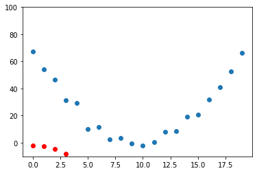
preds = f(time, params)  # Calculate the predictions


def show_preds(preds, ax=None):
    if ax is None:
        ax = plt.subplots()[1]
    ax.scatter(time, speed)
    ax.scatter(time, to_np(preds), color="red")
    ax.set_ylim(-10, 100)


show_preds(preds)

14.3

Calculate the loss
E.g.,

loss = mse(preds, speed)
loss

tensor(23193.9277, grad_fn=<MeanBackward0>)

14.4

Calculate the gradients

loss.backward()
params.grad

tensor([-50335.4492,  -3227.3774,   -239.5752])

params

tensor([-0.7772,  0.3563, -2.0146], requires_grad=True)

14.5

Step the weights $\iff$ Update the parameters

lr = 1e-5
params.data -= lr * params.grad.data
params.grad = None  # grad is by default None and becomes a tensor the first time a call to `backward()` computes gradients for `self`.

14.5.X

What is attribute propertyTensor.grad by default?
What, after the first call to backward()? What needs to be added, when calling backward()?
What information will it hold after the first call to backward() and update continuously?

.grad is None by default
After the first call to backward(), it becomes a tensor. The gradient is calculated for self, by backward().
The attribute will then contain the gradients computed and future calls to backward() will accumulate (add) gradients to it.

Automation for several steps can be added by using something like the function below and for x in range(10)

lr = 1e-5


def apply_step(params, prn=True):
    preds = f(time, params)
    loss = mse(preds, speed)
    loss.backward()
    params.data -= lr * params.grad.data
    params.grad = None
    if prn:
        print(loss.item())
    return preds

14.6

Iterate and improve the predictions of the model through performing the stochastic gradient descent over a specified number of epochs.

for i in range(10):
    apply_step(params)

70654296875
448974609375
7951049804688
1010131835938
69140625
2589111328125
4173583984375
2552490234375
2217407226562
2125244140625

Progress can be monitored by plotting the results before and after a step has been made.

14.7

Stop
- Stop after a certain amount of epochs.
- Stop after a certain threshold for the loss function has been achieved.

15.

How do we initialize the weights of a model?

They are initialized randomly, have random values.

param = torch.randn(10).requires_grad_()
param

tensor([-0.1867,  0.7082, -1.3939,  1.3704,  0.4547,  0.3694,  0.2572,  0.2377,
        -1.1686,  0.1628], requires_grad=True)

16.

What is ‘loss’?

Loss is a value, that we get during the Stochastic Gradient Descent process.
Loss tells us how well or badly our model is doing.

17.

Why can’t we always use a high learning rate?

If the learning rate is too high, it might happen that we don’t follow the gradient towards the minimum, but that we jump to another section of the function. This could be a spot, that is not closer to the minimum. Subsequent steps can repeat this ‘bouncing around’ behavior.

18.

What is a gradient?

A gradient, as it is used in deep learning during the SGD, is the value of the first partial derivative at a certain point of the loss function.
We calculate the first partial derivative of the loss function
($\frac{d}{dw_{i}}$)for all weights $w_{i}$,$i \in N$, with $N$ the total number of weights.
The gradient then is, for each $w_{i}$:$\frac{d}{dw_{i}}$$.
The gradient, with the steepest slope is chosen for the stepping, which is equivalent to the one, that fulfils: $max_{i \in N}(\,|\frac{d}{dw_{i}}|)\,$. Which can be represented by a vector with $N$ elements, each element is a number that is given by the first partial derivative of the loss function, at the most recent value for each weight in the total of $N$ weights.

19.

Do you need to know how to calculate gradients yourself?

No, the deep learning library does the computation.
However, you do need to understand what the ‘gradient’ value means for the SGD - that is where the SGD is at each step of the SGD.
The calculation is simple, most of the time and only requires one to use the chain rule.
At each step, one needs to understand the values derived from calculating the first partial derivative of the loss function and how they interact with the learning rate, the stepping function, during the actual stepping - and where the stepping leaves one.

20.

Why can’t we use accuracy as a loss function?

The accuracy function ($f$in the following) is a binary function, that summarizes all predictions ($preds$), that have been made by the model during a step in the SGD and assigns an integer representation for each prediction in$preds \in {0,1}$. If the single prediction$pred$is correct, it assigns a$1$, $0$ otherwise. It then divides that sum by the total of $pred$ in $preds$. So it returns, the fraction of correct predictions out of all the predictions made. The partial derivative of $f$ is always $$0$, which makes it unsuitable for any type of the Gradient Descent, which relies on the gradient of the loss function at every step of the optimization to guide it towards finding at least a local minimum. Finding the global minimum is not guaranteed, when using SGD (it is the same for GD), but a local minimum can still deliver a ‘good enough’ result. The gradient of the loss function should reflect small changes in the values of the weights.

These are the reasons, why accuracy is not a suitable loss function to drive the optimization. It does however make for a good metric, that is meant for human understanding of how well or badly the model is doing, calculated at the end of every epoch for the predictions of the model on the validation set.

21.

Draw the sigmoid function. What is special about its shape?

The sigmoid function maps any input to the interval $[0,1]$.
It is monotonously increasing and it can be specified, over which $x$ range the output goes from 0 to 1.
Since it is monotonously increasing, once output reaches 1, its output will remain 1 for all subsequent $x$ values.
Unlike some of the other activation functions, the sigmoid function is differentiable over its entire domain.
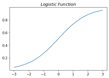
An example of a popular activation function is the $Logistic$ function.
The sigmoid function can look like this, in the case of the $Logistic$ function:

import fastbook

fastbook.setup_book()
from fastbook import *

def sigmoid(x):
    return 1 / (1 + torch.exp(-x))

plot_function(torch.sigmoid, title="$Logistic\,\,Function$", min=-3, max=3)

22.

What is the difference between a loss function and a metric?

Loss Function
- Is used to drive the SGD $\iff$ The automated learning process on the training dataset
- Needs to be differentiable
- Needs to be reasonably smooth
  - Must not have long flat sections
  - Must not have large jumps
  - Must respond to small changes in the predictions of the model

Metric
- Used for human understanding of ‘how well the model is doing’, in terms of achieving the overall objective.
- Is calculated on the validation dataset, on for the model unseen data that is.
- Typically, is computed after each training epoch.

23.

What is the function to calculate new weights using a learning rate?

The function for each update step looks like this:

\[w_{i} = w_{i} - lr \frac{d}{dw_{i}}L(\,w)\,\]

Let $I$ be the set of weights (in fact the set of all parameters in the network) in the network, and $w_{i} \in I$ a single weight. Then the updated weight $w_{i}$, is given by the partial derivative of the loss function$L$with respect to$w_{i}$, multiplied by the learning rate $lr$, which is then subtracted from the value of weight$w_{i}$, prior to the update.

24.

What does the DataLoader class do?

The DataLoader class helps us in keeping some of the factors during training continuously changing, which is beneficial for the training outcome.
The DataLoader class does the minibatch creation for us.
- It randomly shuffles and collates random sample for each step in the SGD.
It can take any Python collection and turn it into an iterator over minibatches, like so:

# Each tensor can only have 10 elements at maximum, it seems?
coll = range(36)
for i in range(10):
    dl = DataLoader(coll, batch_size=10, shuffle=True)
    print(list(dl))

[tensor([15, 34, 10, 19, 30, 14, 22, 20, 29,  4]), tensor([26,  0, 33, 23, 31,  7,  5, 35, 27,  3]), tensor([28, 18, 12, 13, 17, 11, 16, 21,  6,  8]), tensor([ 1, 25, 24,  9,  2, 32])]
[tensor([35, 21, 16, 28, 32, 15,  9, 13,  8, 25]), tensor([30, 18, 12, 11, 20, 34, 31, 10,  3, 23]), tensor([ 2,  0, 33, 22,  6,  5,  7, 17, 26, 29]), tensor([24,  1, 14,  4, 27, 19])]
[tensor([28,  1, 35, 24, 34,  8,  9,  3, 33, 12]), tensor([29, 14,  2, 25,  4, 26, 10, 11, 30,  5]), tensor([22, 20, 23, 18,  6,  7,  0, 31, 21, 13]), tensor([27, 17, 32, 15, 19, 16])]
[tensor([17,  4, 10, 25, 28, 15, 16, 11,  3, 34]), tensor([23,  0, 31, 12, 20,  9,  7, 27, 29,  6]), tensor([24, 30, 35, 14, 22, 26,  2,  1, 18,  8]), tensor([19, 32, 21, 33,  5, 13])]
[tensor([14,  8, 10, 15, 27, 13,  0,  6, 29, 20]), tensor([ 2, 11, 16, 34, 17, 21, 32,  3, 12,  4]), tensor([30,  9, 24, 23, 25, 26,  5, 33,  1, 19]), tensor([28,  7, 35, 18, 31, 22])]
[tensor([ 7, 33, 17, 15,  5, 10,  8, 25,  4, 14]), tensor([ 3,  6, 28, 21, 11, 19, 22,  0, 16, 23]), tensor([31, 29,  1,  9, 32, 27, 30,  2, 18, 20]), tensor([13, 24, 34, 12, 35, 26])]
[tensor([ 1, 31, 16, 23, 32, 19,  7,  6,  2, 35]), tensor([24, 30, 10, 34, 26, 28, 18, 13, 22, 15]), tensor([ 0, 27,  3, 14,  4, 33, 29,  8, 25, 11]), tensor([ 5, 12, 20, 21, 17,  9])]
[tensor([12, 29, 25, 31, 34, 11,  0, 21, 16, 28]), tensor([ 2, 27,  6, 17, 15,  1, 14,  3, 18,  8]), tensor([23, 24,  9, 26, 13, 35, 22, 20, 30, 33]), tensor([32, 19, 10,  4,  5,  7])]
[tensor([11, 12, 18, 26, 27, 34, 33, 16,  9,  7]), tensor([29,  3,  0, 25, 19, 30, 22,  1, 31, 15]), tensor([13,  2, 20, 24, 10, 17, 28, 14,  8, 35]), tensor([23,  4,  5, 21, 32,  6])]
[tensor([10, 18, 17, 31,  8,  9,  0, 24, 34, 12]), tensor([35,  6, 19, 21, 16, 28, 20, 30, 22,  3]), tensor([ 4, 25, 11, 32,  5, 13, 29, 26, 14, 23]), tensor([27,  1, 15, 33,  7,  2])]

A DataLoader can take a Dataset as input:

ds = L(enumerate(string.ascii_lowercase))
print(ds)
dl = DataLoader(ds, batch_size=6, shuffle=True)
print(
    list(dl), "\n"
)  # DataLoader needs to be transformed from DataLoader to list() object
print(list(dl)[0])  # testing Black

[(0, 'a'), (1, 'b'), (2, 'c'), (3, 'd'), (4, 'e'), (5, 'f'), (6, 'g'), (7, 'h'), (8, 'i'), (9, 'j'), (10, 'k'), (11, 'l'), (12, 'm'), (13, 'n'), (14, 'o'), (15, 'p'), (16, 'q'), (17, 'r'), (18, 's'), (19, 't'), (20, 'u'), (21, 'v'), (22, 'w'), (23, 'x'), (24, 'y'), (25, 'z')]
[(tensor([ 1,  4, 21,  5, 17, 24]), ('b', 'e', 'v', 'f', 'r', 'y')), (tensor([23,  9, 22, 13,  2,  6]), ('x', 'j', 'w', 'n', 'c', 'g')), (tensor([16, 12, 14,  7, 20, 15]), ('q', 'm', 'o', 'h', 'u', 'p')), (tensor([ 8, 18,  3,  0, 25, 19]), ('i', 's', 'd', 'a', 'z', 't')), (tensor([11, 10]), ('l', 'k'))] 

(tensor([5, 4, 3, 7, 0, 2]), ('f', 'e', 'd', 'h', 'a', 'c'))

25.

Write pseudocode showing the basic steps taken in one epoch for SGD.

def fp(num):
    params=torch.randn(num)
    return params

def m(dat,params):
    pre = dat*params
    return pre

dat=[1,100,1000,1,200]
tt=[1,1,1,1,0]
lr=1e-5
def ll(pre,tt):
    l=(pre-tt).abs()
    return l

def st(params,lr):
    for p in self.params: p.data -= p.grad.data * self.lr

lu = []
sc = []
for n in range(5):
    params = fp(5)
    lu.append(m(dat[n],params))
    sc.append(ll(lu[n],tt[n]))
    params=st(params,lr)

# define, for each x,y pair in the training set, that is each tuple of (independent variable, dependent variable).
for x,y in dl: 
    pred = model(x) # The 'model' function, that makes predictions based on input x
    loss = loss_func(pred,y) # Loss function, that computes the loss for the previous step in regard to pred and y
    loss.backward() # The calculation of the gradient, based on the loss function
    paramters-= parameters.grad * lr # Updating the parameters after each training loop, by using the standard SGD formula to update the weights

26.

Create a function, that if passed two arguments [1,2,3,4] and 'abcd', returns [(1,'a'), (2,'b'), (3,'c'), (4,'d')]
What is special about that output data structure?

# Answer to first part of the question
a = [*range(1, 5)]
b = [x for x in string.ascii_lowercase[:4]]
print(a, b)


def tt(a, b):
    return list(zip(a, b))


tt(a, b)

[1, 2, 3, 4] ['a', 'b', 'c', 'd']

[(1, 'a'), (2, 'b'), (3, 'c'), (4, 'd')]

What is special about these tuples, is that they can be used to represent a pair of independent variable, dependent variable for each such set in the dataset. Using this tuple structure, one can conveniently access the independent and dependent variable by using standard python indexing. E.g., for a tuple t=(1,'a') , one can access the first component like so: t[0] and the second one, like this: t[1]

27.

What does view do in PyTorch?

view lets one reshape a tensor, much like the numpy reshape function does.
By using view, one can alter all dimensions of a tensor, as long as the total number of elements remains the same.
E.g., A 2D tensor t with dimensions t.ndim = (1,20), can be reordered using view, like so: t.view(2,10) or t.view(10,2) or any other shape where the multiplied shape along its two axes remains 20.

28.

What are the bias parameters in a neural network?
Why do we need them?

In neural networks, the intercept ($b$) in an equation of the form $y=wx+b$ is called bias, together with the weights ($w$) in the example they make up the parameters.
The bias parameters are randomly initiated, like the weights.
We need the bias weights, since they are part of the fundamental linear equation $$y=wx+b$, which is used in any linear layer.

29.

What does the @ operator do in Python?

The @ operator is the matrix multiplication operator in Python.
It can be used to multiply two matrices or two vectors or a vector and a matrix.

The basic rule is, that two objects, any combination of matrix@matrix, vector@matrix, matrix@vector or vector@vector and any chain or permutation of these objects, $M \in \mathbb{R}^{N\mathrm{x}M}$ and $N \in \mathbb{R}^{M\mathrm{x}M}$ must have matching inner dimensions for a matrix multiplication to be possible. Here, the right most dimension of $M$ and left most dimension of $N$ need to match. If this is the case, the product of M@N = Q will have dimensions $MN=Q \in \mathbb{R}^{N\mathrm{x}M}$, which is equal to the outer dimensions of$M$and$N$$.

30.

What does the backward method do?

the backward method refers to back propagation, which is the name to the process of calculating the derivative of each layer.

yt=f(xt)
yt.backward()
xt.grad

31.

Why do we have to zero the gradients?

The gradients, that have to be zeroed (using PyTorch’s in place operations here) are the ones of the:
- weights, by weights.grad.zero_()
- bias, by bias.grad.zero_()
The reason, the gradients need to be set to zero, is that loss.backward() adds the gradients of loss, also known as L(w) to any gradients that are currently stored.
Because loss.backward() stores the gradients for all weights $$w_{i}$, one needs to empty the stored gradients before each new training epoch.

32.

What information do we need to pass to Learner?

Learner is a class found in the fastai library. From the fastai docs:

Learner: A basic class for handling the training loop

The following inputs need to be specified, when creating an object of class Learner:

dls is a DataLoaders object, which can be created from standard PyTorch dataloaders or preferably from classes from within the fastai library.
model is any valid model from within PyTorch or fastai. E.g., nn.Linear(28*28,1).
opt_func is the optimization function. E.g., SGD.
loss_func is the loss function. E.g., MSE, MAE or a custom loss function.
metrics is the metric to use to evaluate model performance after each epoch. E.g., batch_accuracy.

Additional parameters and their default values, where applicable are:

parameter	explanation	example	default
`lr`	learning rate	0.0001	0.001
`splitter`	function, that takes `self.model` and returns a list of parameter groups		`trainable_params`
`cbs`	is one or a list of `Callback`s to pass to the `Learner`. `Callback`s are used for every tweak of the training loop. Every `Callback` is registered as an attribute of `Learner`.
`path`/`model_dir`	`path` and or `model_dir` are used to load/save models. Often `path` will be inferred from `dls`.
`wd`	`wd` is the default weight decay used when training the model.
`moms`	`moms` are the default momentums used in `Learner.fit_one_cycle`
`wd_bn_bias`	`wd_bn_bias` controls, if weight decay is applied to `BatchNorm` layers and bias.	True or False	False
`train_bn`	`train_bn` controls, if `BatchNorm` layers are trained even when they are supposed to be frozen according to the `splitter`. Our empirical experiments have shown that it’s the best behavior for those layers in transfer learning.

33.

Show Python or pseudocode for the basic steps of a training loop.

This is an example of how the basic steps of a training loop can look like (It was a try, see pseudo code solution following it):

# define underlying function, that is unknown to the model.
from scipy.stats import expon, norm

day_g = np.random.default_rng()
day_alphas = np.abs(day_g.normal(loc=8, scale=4, size=100))
night_alphas = np.abs(day_g.normal(loc=16, scale=3, size=100))
# print(f'day_alphas is {day_alphas}')
sv_day = [
    [float(np.abs(a + t + s)) for t, a in zip(norm.rvs(size=100), day_alphas)]
    for s in expon.rvs(size=100)
][:100]
sv_night = [
    [
        float((np.abs((a + t ** 2 + s) - 15)) + (a + t - s ** (a * 0.0044)))
        for t, a in zip(norm.rvs(size=100), night_alphas)
    ]
    for s in expon.rvs(size=100)
][:100]
ar = np.append(np.array([sv_day]), np.array([sv_night]))
np.random.shuffle(ar)
ar = ar[:100]
print(len(ar))
print(ar)


def f_d(s, e, l, sv_day):
    return s * sv_day + e ** 1e-4 * sv_day - l


def f_n(s, e, l, sv_night):
    return s * sv_night + e ** 1e-4 * sv_night + 0.4 * sv_night + l


def f_o(s, e, l, sv):
    return s * sv + e ** 1e-4 * sv + 0.4 * sv + l

100
[21.0383076   5.09801729  3.15178782 15.86700732 14.60580718  6.72232093 10.09499213  7.81423959  6.35270302 13.69528753  8.17166694  0.17579181 11.42915517  4.15294509 11.36371436  4.51596443
61617202  9.7052531  17.42816216 12.9961129   1.71536369 15.54351609 26.95205708 20.62786489  2.98404346  1.82134782  2.56090975 13.36052885 28.99409047 23.99459551  7.13222712  8.41815448
9421428   7.26963884 14.4485025  13.42538567 14.81994856 13.92925997 11.04847036  6.26272201 23.4621644  20.3589856  14.99204    16.55806094  0.84962732 19.49579972 21.05035358 23.98173912
31816698 17.24080972 13.56165375 23.2759328   8.8600213  23.2144287  24.32831734  4.70862568 29.50623363 14.02466347 21.16747778  8.84457883  4.66644838 17.96983548 27.27848834 20.60473737
04113639 23.9695169  13.68600503 21.85875209 21.3025661  14.93849819 20.06305356 12.54641644  3.33056871  9.68635345 12.78958228 13.71467483 17.45915385 11.35622196 18.16559036 11.90514113
2044745   8.85681539 17.31016852 38.23133812 17.04967248 23.17025778  9.98671168 14.54430101 22.97475546  6.54350307  9.40580956 14.91655192 20.52040332  8.08800518 11.20310281 17.69301348
16125983 21.41862019  8.56823459 16.94257652]

Looking At The Ten Minute Value

From the test we can see that, for example, the 10-minute mark separates the sv_day and sv_night distributions quite well. There is no value in the sv_night distribution, that is below the 10-minute mark, while roughly half of the values in the sv_day distribution are below it.

for i in [sv_day, sv_night]:
    i = i[0][:100]
    print(f"length is: {len(i)}")
    ss = [1 for s in i if s < 10]
    print(sum(ss))

length is: 100
75
length is: 100
1

Step 1.

Initialize the parameters to random values.

params = torch.randn(3).requires_grad_()
orig_params = params.clone()

Step 2.

Calculate the predictions

def ri():
    id = torch.randn(1) % 20
    return id

preds = f_o(params[0], params[1], params[2], ri())

Step 3. Calculate Loss

def lmse(preds, ar, i):
    ari = ar[i]
    loss = ((preds - ari) ** 2).abs().mean()
    return loss

Step 4.

Calculate the gradients

lmse.backward()
params.grad
lr = 1e-5

Step 5.

Step The Weights

params.data -= lr * params.grad.data
params.grad = None
preds = f_o(s, e, l, ar)
lmse(preds, sv_night)

def apply_step(params, prn=True):
    preds = f_o(s, e, l, ar)
    loss = lmse(preds, sv_night, i)
    params.data -= lr * params.grad.data
    params.grad = None
    if prn:
        print(loss.item())
    return preds

Step 6. Repeat The Process

for i in range(10):
    apply_step(params)

34.

What is ‘ReLU’?
Draw a plot of it for values from -2 to 2.

‘ReLU’ is an abbreviation for rectified linear unit and is a type of activation function.
An activation function manages the outputs of a layer, as they are passed on to the next layer or as output of the final layer.
It determines, if a layer gets activated by an input (gets active and passes on something) or not.
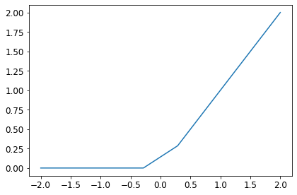
The ‘ReLU’ function is given by the following definition:

\[\mathrm{ReLU}(\,x)\,\,=\,\mathrm{max}(\,0,x)\,\]

It can be defined and plotted for the values between -2 and 2, like so:

def ReLU(x):
    return max(0, x)


ReLU(1)

1

x = np.linspace(start=-2, stop=2, num=8, endpoint=True)
rx = [ReLU(j) for j in x]
print(rx)
fig, ax = plt.subplots(1, 1, figsize=(6, 4), tight_layout=True)
ax.plot(x, rx)
plt.title = "Plot of ReLU function"
ax.set_ylabel = "ReLU Function"
plt.show()

[0, 0, 0, 0, 0.2857142857142856, 0.8571428571428568, 1.4285714285714284, 2.0]

png

35.

What is an activation function?

In neural networks, input values are typically continuous, and nodes take continuous inputs and produce continuous outputs.
Some of the inputs to nodes are parameters of the network; the network learns by adjusting the values of these parameters so that the network as a whole fits the training data.
Each node within a network is called a unit.
Traditionally, following the design proposed by McCulloch and Pitts (Perceptron Mk 1), a unit calculates the weighted sum of the inputs from predecessor nodes and then applies a nonlinear function to produce its output.
Let $a_{j}$ denote the output of unit $j$ and let $w_{i,j}$ be the weight attached to the link from unit $i$ to unit $$j$; then we have:

\[a_{j} = g_{j}(\,\sum_{i}w_{i,j}a_{i})\, \iff g_{j}(\,{in}_{j})\,,\]

where $g_{j}$ is a nonlinear activation function associated with unit $j$ and ${in}_{j}$ is the weighted sum of the inputs to unit $j$.

Annex To 35.

The fact that the activation function is nonlinear is important because if it were not, any composition of units would still represent a linear function. The non-linearity is what allows sufficiently large networks of units to represent arbitrary functions. The universal approximation theorem states that a network with just two layers of computational units, the first nonlinear and the second linear, can approximate any continuous function to an arbitrary degree of accuracy. The proof works by showing that an exponentially large network can represent exponentially many “bumps” of different heights at different locations in the input space, thereby approximating the desired function. In other words, sufficiently large networks can implement a lookup table for continuous functions, just as sufficiently large decision trees implement a lookup table for Boolean functions. ~p. 1383 ai modern approach.

36.

What is the difference between F.relu and nn.ReLU?
nn.ReLU is a PyTorch module, that does the same thing as the F.relu function.
Most functions that can appear in a model also have identical forms that are modules.
Generally, it is just a case of replacing F with nn and changing the capitalization.
When using nn.Sequential, PyTorch requires us to use the module version.
Since modules are classes, we have to instantiate them, which is why you see nn.ReLU() in this case.
Since nn.Sequential is a module, we can get its parameters, which will return a list of all the parameters of all the modules it contains.
What is a heuristic, that describes a relationship between number of layers in a model and the choice of learning rate and epochs?
The more layers a model has, the lower the learning rate and the fewer epochs are used for fitting the model.

37.

The universal approximation theorem shows that any function can be approximated as closely as needed using just one non-linearity. So why do we normally use more?
The universal approximation theorem shows, that by using a nonlinear first layer, and a linear second one, can approximate any continuous function to an arbitrary degree of accuracy.
The proof works by showing that an exponentially large network can represent exponentially many ‘bumps’ of different heights at different locations in the input space, thereby the desired function.
In other words, sufficiently large networks can implement a lookup table for continuous functions, just as sufficiently large decision trees implement a lookup table for Boolean functions.
The reason most networks have more layers, is that while it is possible to approximate any continuous function in theory, in practice the following problems often occur when following the architecture used in the universal approximation theorem:
- The result is a model, that uses a huge parameter matrix, that section-wise defines the output function used to approximate the continuous function.
- The generalization capabilities of such a model, often are very limited.
- Such a parameter matrix (size of the matrix is proportional to the total number of parameters used in the model) requires large amounts of memory and can cause problems, if there is not enough memory to store it in.
- Deeper models show higher performance, as they possess the following characteristics:
  - Adding more layers, means that fewer parameters are needed in the model.
  - That means smaller parameter matrices.
  - That in turns leads to quicker fitting.
  - Less memory intensive, compared to the large parameter matrix models.
  - Models, that only use one nonlinear layer are very rare nowadays.